We can study derivatives in two ways: at a specific point or as a function defined for every point where the derivative exists.
The derivative of a function at a point is nothing other than the slope of the tangent line to the graph at that specific point.
The derivative function assigns to each point the slope of the tangent line to the graph at that point. It allows us to determine where the original function is increasing or decreasing, locate extrema, and analyze its behavior.
Before we start calculating derivatives, it is important to keep in mind that a function is differentiable at a given point if the following limit exists and is finite:
x→x0limx−x0f(x)−f(x0). Although this definition allows us to calculate derivatives directly, in most cases we use derivative rules that make calculations significantly faster and easier, which will be introduced later.
This becomes much easier to understand when you look at the graphical interpretation.
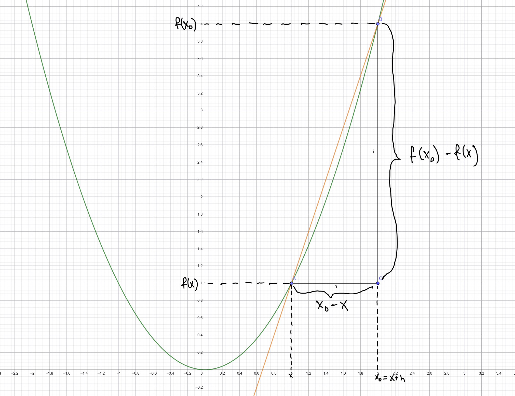
Geometrically, a derivative represents the slope of a tangent line to a curve at a given point. If we take two separate points on a graph, the fraction below calculates the slope of the line passing through them (called a secant line).
By applying a limit, we bring these two points infinitely close to each other. As the distance between them shrinks to zero, the secant line transforms into a tangent line. This process can be expressed using one of the following two equivalent definitions:
x→x0limx−x0f(x)−f(x0) or h→0limhf(x+h)−f(x)
, but we will use the first one in most cases for easier calculations.
However a function is differentiable on its domain if it is differentiable at every point of that domain. Intuitively, a function fails to be differentiable whenever the limit defining the derivative does not exist as a finite number. This often happens at discontinuities, sharp corners, cusps, or vertical tangents.
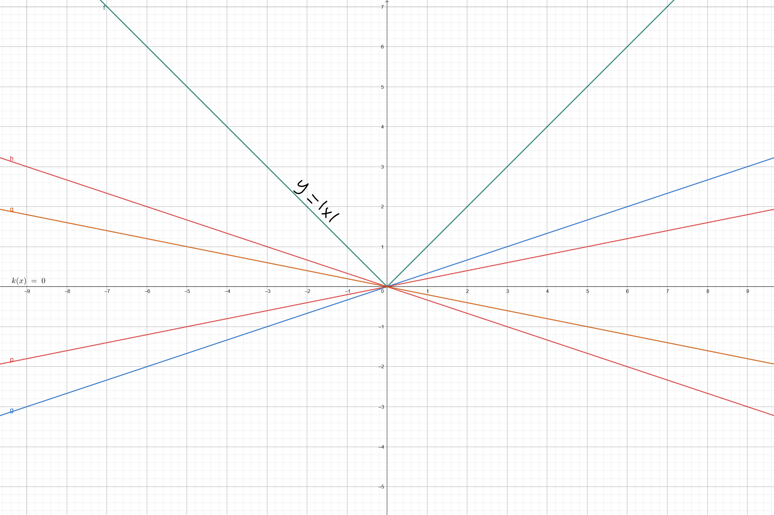
One situation where this condition is not met is when the graph has a sharp shape—such as the absolute value function ∣x∣ at x=0. It is not hard to see that the function ∣x∣ could have several different tangent lines at this exact point.
In the next sections, we will start by learning how to calculate derivatives of simple functions, meaning functions that are not composed of any other functions and depend only on themselves. Then, we will explain how to differentiate composite functions.
After that, we will learn how to analyze a function using its derivative, how to find extrema, what they mean, and what information the derivative gives us about the behavior of the function.
Finally, we will calculate the derivative at a specific point and determine the tangent line at that point. We will leave this topic until the end because calculating the tangent line requires finding the derivative of the function first.
The Derivative Function
How Do We Find the Detrivative Function?
You could say that we simply use ready-made formulas. Depending on whether our function consists of basic elementary functions or is a composition of several different functions, we apply the appropriate rules. When it comes to basic elementary functions, we use the following standard formulas:
These formulas come from the definition of the derivative:
limx→x0x−x0f(x)−f(x0) or limh→0hf(x+h)−f(x)
We will use the first definition throughout this article because it is usually easier to work with.
Both definitions yield the exact same result. The idea behind deriving derivative formulas is that we start by choosing an arbitrary point x0
and calculate the derivative at that point. The reason we can later write the result using the variable x instead of the notation x0 is that x0 was not a specific point,
it represented any point from the domain of the function. For example, if after calculating the limit we obtain: f′(x0)=2x0,
this means that the derivative at any chosen point is equal to twice the value of that point. Since the point x0 could have been any point, we can write the general derivative function as: f′(x)=2x,
The symbol changes, but the meaning stays the same: it describes the derivative at an arbitrary point of the function.
Now, let’s calculate the derivative of the function f(x)=x2 using the limit definition. Substituting it into our formula, we get:
limx→x0x−x0x2−x02=limx→x0x−x0(x−x0)(x+x0)=limx→x0(x+x0)=2x0=2x
Now, we can generalize this method for the power function f(x)=xn. Using the algebraic identity for the difference of n-th powers, we can expand the limit as follows:
Evaluating the limit by substituting x=x0, each term in the expression transforms:
=x0n−1+x0n−2x0+x0n−3x02+⋯+x0x0n−2+x0n−1
=x0n−1+x0n−1+x0n−1+⋯+x0n−1+x0n−1=nx0n−1
Why do we end up with exactly n identical terms of x0n−1? If we closely examine the expression inside the limit, we can track the powers of x0 across the sequence. In the first term, the power of x0 is 0, so x00=1 (leaving us with xn−1), in the second term we have x01=x0, and this pattern continues all the way up to the final term x0n−1. This forms a sequence of exactly n elements.
At this point, we have obtained the expression in terms of x0n−1 rather than xn−1. Since x0 was chosen as any arbitrary point, we can replace it with a general variable x, which gives us the final derivative formula: (xn)′=nxn−1.
Following this idea, we can derive many of the formulas from our table, although some functions require additional techniques.
Why Do We Use the Derivative Function?
The derivative function allows us to determine the monotonicity of the original function. In other words, it tells us how the values of the original function (the function from which we calculated the derivative) change. A derivative also allows us to determine the points at which the original function has an extremum, meaning either its maximum or minimum value.
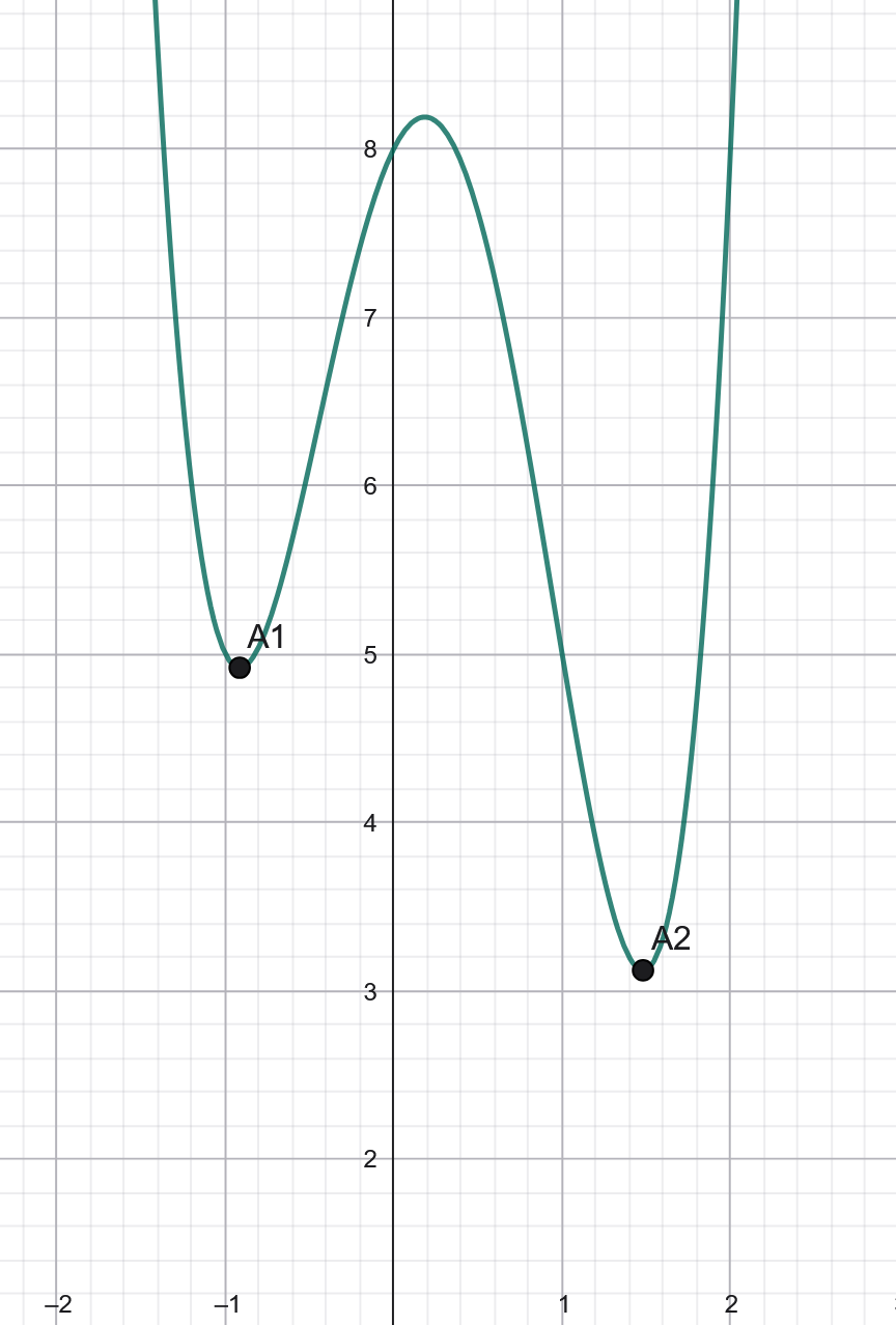
An extremum can be local or global. For example, consider the polynomial: 2x4−2x3−5x2+2x+8.
Looking at the graph, we can see that point A1 is a local extremum, more specifically a local minimum. This is because if we move a small distance to the left or to the right of point A1, the value of the function at A1 is lower than the values at the nearby points. However, A1 is not the global minimum. If we look at point A2, we can see that the polynomial reaches its lowest value there. Therefore, A2 is the global extremum, more precisely the global minimum. It is also worth noting that A2 is a local minimum as well.